The splicing predictors Pangolin and SpliceAI recovered 65 and 64 positive variants in their respective top 100 MFASS predictions. Yet a recall diagnostic put SpliceAI slightly ahead: 20.78% against 20.70%. Restricting the comparison to variants both methods scored put Pangolin ahead: 21.10% against 20.78%. Each method retained exactly its own original selections. The denominator alone changed the order. Evidence audit.
This was a diagnostic we added during research, recall_at_capacity. Rewire's biology benchmark database already reported precision at 100. That result remained 65% versus 64%; the database contained no recall field to reverse. The finding explains a comparison without overturning the database leaderboard. Metric provenance.
Our first AI-assisted investigation examined four human-selected benchmark cases and controls. Two other checks found a constant predictor scoring above 0.92 on a ranking metric and another receiving perfect top recall. Inspecting the populations and evaluator rules explained these results. The findings are methodological; no new biological mechanism has been established. Campaign records, quantitative audit.
Recall needs a named population
MFASS tests how genetic variants affect exon recognition in an experimental reporter. Exons are portions of an RNA transcript retained during splicing. A positive label here means assay-defined splicing disruption, not a clinical diagnosis or an effect established in every tissue. Pangolin and SpliceAI predict splicing from sequence. MFASS study, Pangolin study, SpliceAI study.
Suppose follow-up experiments can examine 100 variants. Precision is the fraction of those selected variants that are positive. Recall is the fraction of all positives in a specified population that the selections recover. A fixed capacity fixes the precision denominator; it does not fix the recall denominator. Precision definition, recall definition.
Our eligible test cohort contained 8,324 variants and 315 positives. Every SpliceAI-scored variant also had a Pangolin score, but Pangolin scored additional variants. The table gives the exact counts behind both population choices. Reproduced counts.
| Evaluation population | Method | Scored variants | Positives | Hits in top 100 | Recall |
|---|---|---|---|---|---|
| Own scored rows | Pangolin | 8,301 | 314 | 65 | 20.70% |
| Own scored rows | SpliceAI | 8,194 | 308 | 64 | 20.78% |
| Common rows | Pangolin | 8,194 | 308 | 65 | 21.10% |
| Common rows | SpliceAI | 8,194 | 308 | 64 | 20.78% |
Diagnostic recall at capacity 100. Each method retains its own selected set across population definitions; this does not mean the methods select identical variants. Source: aggregate results.
Matching removed 107 Pangolin-scored variants, including six positives. None was in Pangolin's top 100. Six positives that it had not selected ceased to count in its recall denominator. No tie spanned either whole-population cutoff, so ambiguous tie breaking cannot explain the reversal. Membership and cutoff audit.
The membership check matters independently of the arithmetic. Equal hit counts before and after filtering would not prove that the same variants were selected: one positive could replace another. The later audit compared the selected identities themselves. The 100th and 101st scores were 0.55 and 0.54 for Pangolin, and 0.67 and 0.66 for SpliceAI. Membership and cutoff audit.
The diagram separates the excluded variants from the selections that stayed fixed.
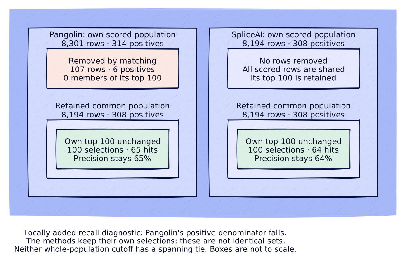
Matching changes Pangolin's positive denominator while preserving each method's own selections. Source: evidence audit.
The original recalls are conditional on each method returning a score. The matched recalls are conditional on both doing so. The latter answers a paired-subset question, but excludes 130 eligible test variants. An unscored variant is not a negative assay outcome. A prospective application needs an explicit missing-prediction policy and coverage report alongside either comparison. Population audit.
Matching rows also leaves differences in input sequence context unresolved. One additional recovered positive does not establish statistical superiority. The exact conclusion is that these saved predictions exhibit a denominator-driven reversal of this particular recall diagnostic. Comparison limits.
For someone selecting candidates from the full cohort, missing predictions may need to remain visible as candidates that could not be ranked. For someone comparing ranking behavior on supported inputs, the intersection may be appropriate. Neither decision can be recovered from the recall number alone. Stating the intended population makes the comparison usable.
The divisions are small enough to check without assay data.
from fractions import Fraction
# Supplied aggregates do not verify labels or selected membership.
hits = (65, 64)  # Pangolin, SpliceAI
own_positives = (314, 308)
common_positives, capacity = 308, 100
own = tuple(Fraction(h, p) for h, p in zip(hits, own_positives))
common = tuple(Fraction(h, common_positives) for h in hits)
precision = tuple(Fraction(h, capacity) for h in hits)
assert own[0] < own[1] and common[0] > common[1]
assert precision == (Fraction("0.65"), Fraction("0.64"))
for label, values in (("Own recall", own), ("Common recall", common), ("Precision", precision)):
    print(label + ": " + ", ".join(f"{float(v):.2%}" for v in values))
Own recall: 20.70%, 20.78%
Common recall: 21.10%, 20.78%
Precision: 65.00%, 64.00%
Arithmetic inputs: aggregate results. These divisions reproduce the ordering; verifying sample identities and unchanged membership requires additional evidence described in the reproduction guide.
A constant predictor scored 0.921 NDCG
The FLIP2 case used 184 test examples from the Rhomax by_wild_type split. Its target is rhodopsin absorption wavelength, where a light-sensitive protein absorbs most strongly. A larger wavelength is not universally better biological performance. Rhomax study, local counts.
Our composition baseline was a simple regression using amino-acid fractions, with a fixed ridge penalty that limits fitted coefficient size. It used no pretraining. A separate control predicted the mean of 584 training targets for every test example. Composition received NDCG 0.954820; the constant received 0.920667, a difference of 0.034153. Baseline metadata, control results.
NDCG means normalized discounted cumulative gain. It sums target-derived gains along a predicted ranking, weights earlier positions more heavily, and divides by the gain from an ideal ordering. The pinned FLIP evaluator subtracts the minimum target, uses the shifted values as linear gains, and includes the full list with logarithmic discounts. Its scikit-learn calculation averages over tied prediction orderings. FLIP evaluator, versioned ranking implementation.
When every prediction ties, the expected gain at each position is the mean gain. Multiplying that mean by the sum of discounts gives expected discounted gain of 3219.780348. Ideal discounted gain is 3497.226700. Their ratio reproduces the constant score. A finite random permutation can differ from this tie-averaged expectation. Audited derivation.
Both controls scored all 184 test examples, so unequal coverage did not explain their difference. Replaying the saved scores and fitting the training-mean control also failed to support a stale-evidence explanation. Those checks narrow the explanation without attributing it to any molecular property. FLIP2 investigation record.
Normalization compares the result with an ideal ordering. It does not subtract the no-information expectation. Here that expectation already approaches the ideal, so the constant reference belongs beside the composition score.
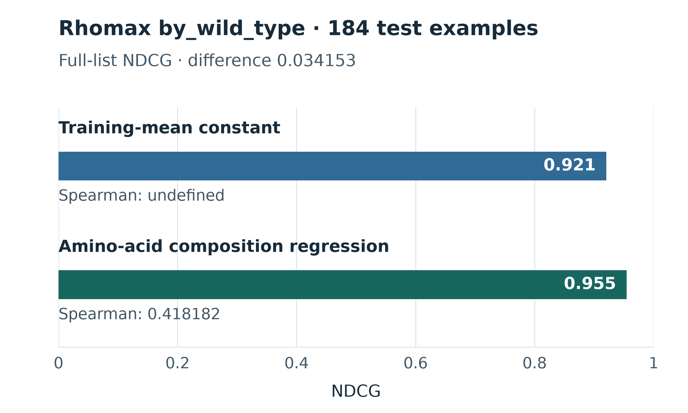
Full-list NDCG with minimum-shifted linear gains, logarithmic discount and tie averaging. The constant calculation is 3219.780348 / 3497.226700 ≈ 0.920667. Source: reproduction results.
Composition did contain ordering information: its Spearman rank correlation was about 0.418. Constant Spearman was undefined because its predicted ranks had no variation. The chosen constant's numerical value cannot affect its all-tied ranking. This establishes a reference for one split and evaluator; 0.955 here is not 95.5% accuracy. Evidence audit.
A percentile threshold selected every row
The ProteinGym control concerned one assay, AMFR_HUMAN_Tsuboyama_2023_4G3O, containing 2,972 rows. Its evaluator defines predicted-top membership using scores greater than or equal to their 90th percentile. The measured top group uses the corresponding threshold on targets. Local counts, pinned ProteinGym evaluator.
For constant predictions, the 90th percentile equals every prediction. All 2,972 rows pass. This includes all 298 true-top observations, producing Top_recall = 1.0 without ranking information. The selected count makes the perfect recall understandable. Control audit.
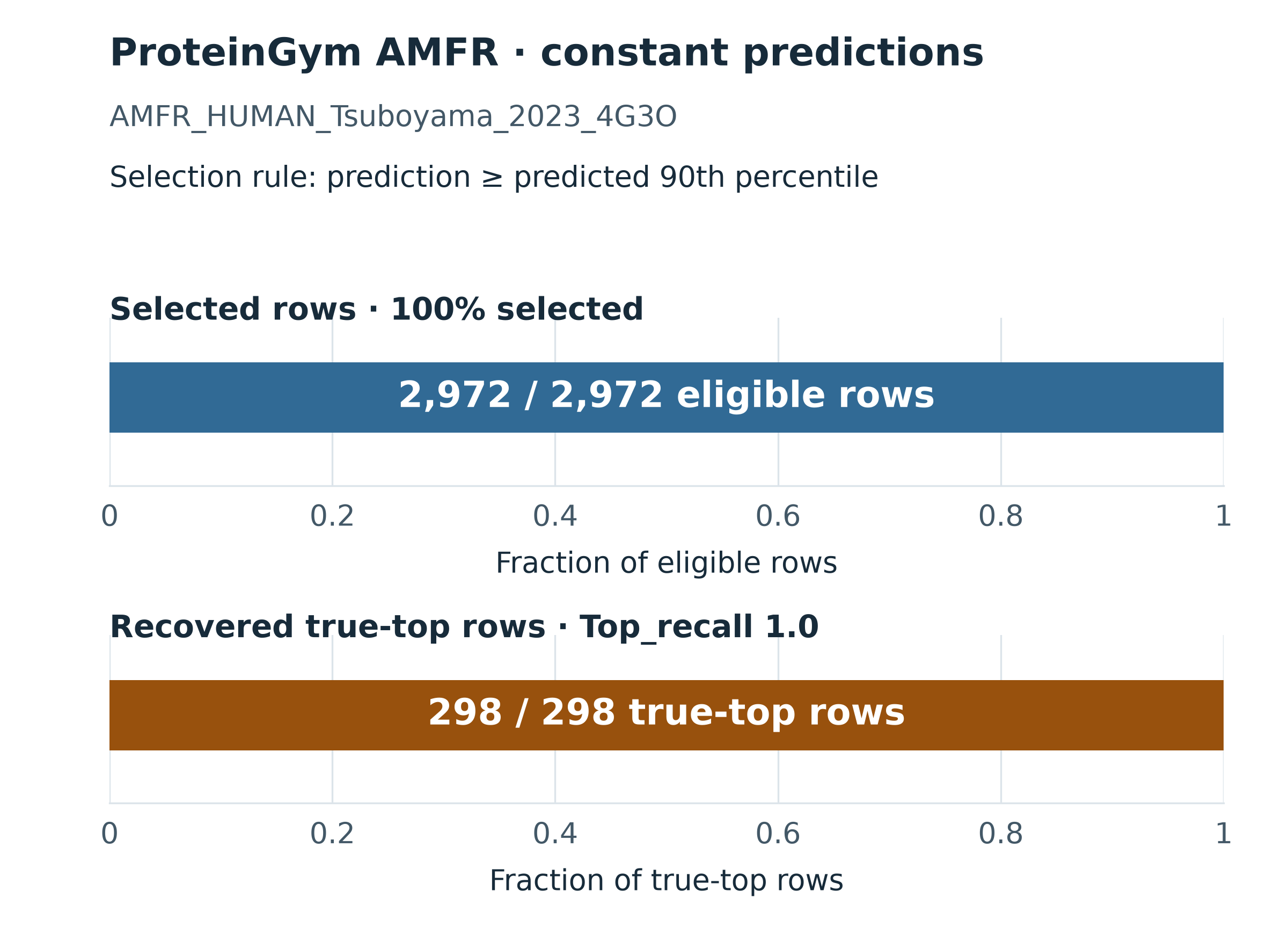
Inclusive percentile selection admits the entire assay under constant predictions. Selection and recall have different denominators. Source: aggregate results.
For a fixed experimental budget, I would report selected count and precision beside recall, then specify an exact capacity and label-independent tie policy. Correlation provides complementary information. These are proposed evaluation choices, not a repair tested in this pilot.
The two constant controls expose different operations. Rhomax's tied items all contribute position-discounted gains; AMFR's ties expand the selected set. ProteinGym also implements a top-decile NDCG distinct from FLIP's full-list calculation. This single-assay observation establishes neither suite-wide failure nor deliberate gaming by submitted models. Evaluator definitions and audit, ProteinGym implementation.
What the AI-assisted process established
People selected the four cases and controls. Separate model calls proposed bounded checks and reviewed interpretations. Plans were frozen before execution; registered code operations performed calculations and recorded receipts. The data had already been inspected, so this was execution registration, not blind scientific preregistration. Campaign records.

Pilot roles and totals come from the campaign records; the subsequent numerical work is documented in the article audit.
One critic caught a sign-direction mismatch: the mRNA plan described composition error minus training-mean error, while the receipt calculated the reverse. Reading the operands resolved the interpretation. We have no human-control comparison showing that AI improved the process overall. mRNA investigation record.
The pilot surfaced the score patterns. The later article audit recomputed saved metrics, verified MFASS selected membership and derived the constant-NDCG calculation. It passed 50 artifact hash checks, 31 metric replays and 64 boundary-band metric checks. Those checks establish consistency of saved evidence; they do not rerun original inference or reconstruct all upstream preparation. The four reports remain pending human scientific review. Audit and limits.
Public aggregate arithmetic is repeatable from the downloadable supplement. Fresh full numerical replay additionally requires exact unpublished derived artifacts, some without public retrieval URLs. The package alone cannot establish which variants were selected or validate the original inference path. Reproduction access.
Unfinished questions also remain visible. The AMFR investigation originally asked whether negative association differed between single and multiple substitutions. No executed mutation-class comparison answered it. A useful control result did not complete that original question. AMFR investigation record.
The next test needs a stronger comparator
MFASS performance varied with distance from annotated exon boundaries. But positive prevalence also changed, from 9.375% within two bases to 1.644% beyond 30. Coverage and sequence context differed, a baseline used distance features, and subgroup cutoffs contained ties. Gene/exon concentration remained unresolved. These descriptive comparisons do not isolate a biological cause. Boundary audit, MFASS investigation.
The mRNABench designed Sample subset offers a more specific next test. Its target is mean ribosome load: measured average ribosome association with assayed mRNA, a translation-related readout rather than direct protein output. Sample study, mRNABench study.
The composition regression uses log-transformed length, A/C/G/T fractions and an unknown-character fraction; RidgeCV selects its regularization strength within training data. Like the protein composition baseline, it has no pretraining. Mean squared error averages squared prediction errors. On the same 15,003 test rows, composition scored 1.91444 versus 2.36553 for the training-fitted global-mean control, about 19.1% lower. Model metadata, reproduced errors.
The pilot did not execute its proposed length or GC outcome comparisons; GC content is the fraction of sequence composed of guanine and cytosine. All test rows were marked duplicate_sequence=no in the prepared table, providing no duplicate-category contrast and no proof that related sequences were separated across the split. mRNA investigation.
A separate post-pilot metadata check found recorded length 855 for every prepared test input. Length strata therefore offer no comparison in this representation. The check did not test outcomes by GC. Feature-coverage receipt.
The global mean tests whether sequence features improve prediction over a constant. The next question is whether composition adds predictive value beyond GC alone. We would fit the composition model and a GC-only baseline on training observations, then compare MSE on identical rows from an untouched cohort of the same mean-ribosome-load task. This comparison remains proposed work.
Before inspecting that cohort, we would define groups of related sequences and assign each whole group to a single partition. We would also set the comparison and decision rules. Persistent incremental improvement would support predictive information beyond GC, not a causal molecular mechanism. Its disappearance would weaken that hypothesis without undoing the observed gain over the global-mean control.
Keep each sample's identifier, measured label, prediction and configuration together. These associations let us reconstruct a population, inspect a cutoff and identify an unexecuted check. Report coverage, positive counts, selection capacity and tie policy beside the score; for ranking metrics, retain the gain definition and no-information control.
References
- Evidence supplement and reproduction access, quantitative audit and aggregate results.
- Evaluator provenance, composition model metadata and post-pilot feature coverage.
- MFASS exon-recognition assay, Pangolin and SpliceAI.
- Rhodopsin absorption-wavelength study, pinned FLIP evaluator and scikit-learn ranking implementation.
- Scikit-learn definitions of precision and recall.
- Pinned ProteinGym evaluator.
- Sample translation assay and mRNABench study.
Help improve this article
Found an error or a better source? Leave a note here, or highlight a passage to comment on it.